
대화형 질의
-> 구조화된 데이터일 경우 사용되는 방법
-> 대표적으로 SQL 언어가 가장 최적화 된 언어.
Operations on structed data
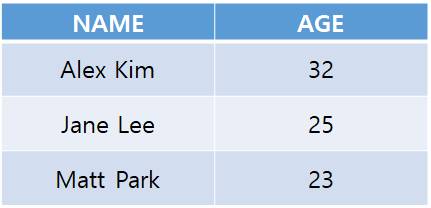
1) Projection
-> 특정 column만 보고 싶을 때 사용
-> E.g., Π[name, age](customer)
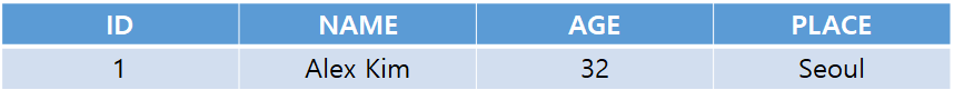
2) Selection
-> 특정 row들만 보고 싶을 때 사용
-> E.g., σage>30(customer)
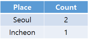
3) Aggreation
-> 하나의 column에 대해 통계를 낸 결과를 보고 싶을 때 사용
-> E.g., Gsum(place)(customer)
4) Join
-> 두 개의 테이블에 있는 데이터를 같이 보고 싶을 때 사용
-> 공통적인 column들의 값이 같은 row를 찾아 병합
- Natural join : 각 두 테이블에 해당하는 column의 값이 다 존재해야 함
- Left outer join : Left 쪽 테이블에 해당하는 column의 값이 있어야 함
- Right outer join : Right쪽 테이블에 해당하는 column의 값이 있어야 함
ex)
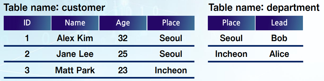
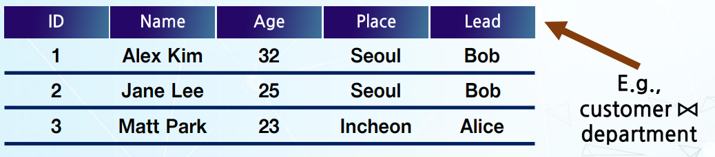
- Natural join (E.g., customer ▷◁ department)
-> Place가 같은 column에 Lead 값 join
대화형 질의를 표현하는 중요한 기능, DataFrame
-> DB의 테이블 or R이나 Python, Pandas에서 사용되는 DataFrame 기능과 비슷하다고 보면 됨.
-> 실제로 Spark에서 SQL을 수행하려면 Spark가 이행하는 RDD 변환으로 바꿔서 수행해야 함

-> Spark Stack에서 Spark SQL을 통해 분석
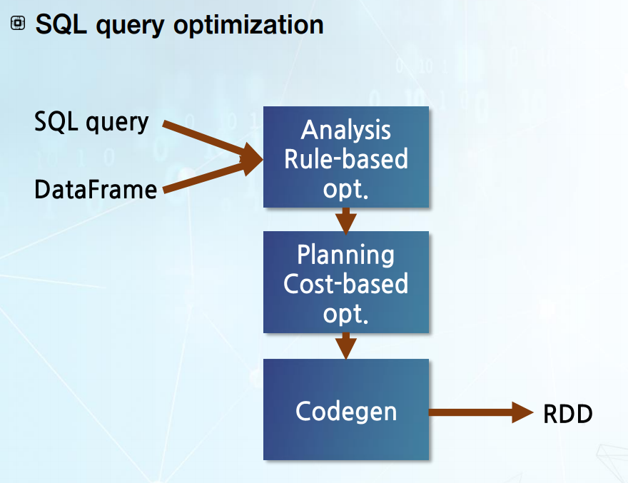
-> SQL 최적화 과정 후 입력으로 SQL질의와 데이터에 해당하는 DataFrame이 들어감
-> 이 분석과정을 통해 최적화된 논리 계획 도출.
-> 그 후 최적화된 논리 계획을 물리 계획으로 만드는 Planning 단계로 들어감(이 단계에서는 Cost 기반의 최적화)
-> 그렇게 나온 SQL 질의 물리 계획은 Codegen이라는 부분에 들어가 Spark가 수행할 수 있는 Spark가 수행할 수 있는 RDD 변환 형태로 바뀜
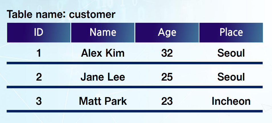
*DataFrame 생성과정
#Read customer data and create a DataFrame
df=spark.read.json("data/customer.json")

#Displays the content of the DataFrame to stdout
df.show()
#┼ ─── ┼ ──────── ┼ ──── ┼ ─────── ┼
#│ id  │   name   │  age │ Place   │
#┼ ─── ┼ ──────── ┼ ──── ┼ ─────── ┼
#│  1  │ Alex Kim │  32  │  Seoul  │
#│  2  │ Jane Lee │  25  │  Seoul  │
#│  3  │ Marr Park│  23  │ Incheon │
#┼ ─── ┼ ──────── ┼ ──── ┼ ─────── ┼

#Print the schema in a tree format
df.printSchema()
#root
#|--id: long(nullable=false)
#|--name: string(nullable=true)
#|--age: long(nullable=true)
#|--place: string(nullable=true)
-> customer.json이라는 데이터를 읽어 DataFrame을 만듦
-> df.show를 통해 DataFrame 내부 정보 중 일부를 택해 standard out으로 보여주게 됨
-> 해당하는 DataFrame Schema가 어떤 형태인지 보고 싶을 때 df.printSchema 사용
위 처럼 만들어진 DataFrame은 여러 operation을 통해 분석 가능하다
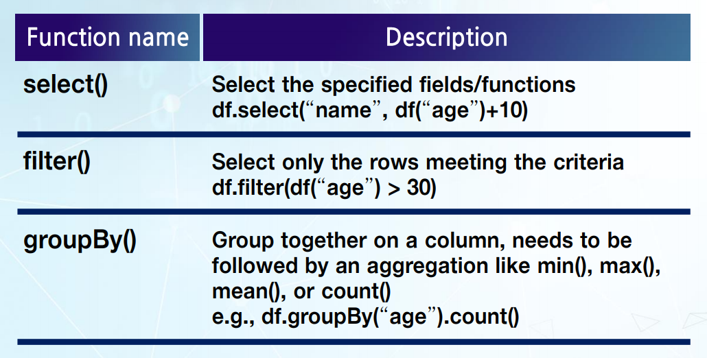
1) select() : 특정 필드와 또는 특정 필드에 함수를 적용한 값을 보여주는 operation
df.select("name", df("age")+10) //name 컬럼 데이터와 age컬럼 데이터에 +10한 결과 (결과적으로 Projection에 해당)
2) filter() : row들 중 특정 조건을 만족하는 row만 선택
df.filter(df("age")>30) // age 컬럼값이 30보다 큰 row만 선택 (결과적으로 Selection에 해당)
3) groupBy() : 어떤 컬럼에 대해 해당하는 column 값이 같은 row들을 모은 후 aggreation 함수 적용
df.groupBy("age").count() // age값이 같은 row가 몇번 일어났는지 age 별로 count를 보여줌 (결과적으로 Aggreation에 해당)
[예제]
#Example1
#select only the "name" column
df.select("name").show()
#┼ ────────── ┼
#│    name    │
#┼ ────────── ┼
#│  Alex Kim  │
#│  Jane Lee  │
#│  Matt Park │
#┼ ────────── ┼

#Example2
#select customers older than 30
df.filter(df['age']>30).show()
#┼ ─────── ┼ ──────── ┼ ──── ┼─ ──── ┼
#│   id    │   name   │  age │ Place │
#┼ ─────── ┼ ──────── ┼ ──── ┼─ ──── ┼
#│    1    │ Alex Kim │  35  │ Seoul │
#┼ ─────── ┼ ──────── ┼ ──── ┼─ ──── ┼

#Example3
#Count customers by age
df.groupBy("age").count().show()
#┼ ───── ┼ ───── ┼
#│  age  │ count │
#┼ ───── ┼ ───── ┼
#│   35  │   1   │
#│   25  │   1   │
#│   23  │   1   │
#┼ ───── ┼ ───── ┼

#Example4
#Join df and df2
df.join(df2, df['name'] == df2['name']).show()
Example1 : DataFrame에서 Name column만 선택해서 결과를 보여줌
Example2 : 이 조건에 만족하는 row를 선택
Example3 : 나이별로 customer가 몇 명 있는지 count
Example4 : df와 df2를 join (name이라는 column을 이용)
Spark SQL
#Register the DataFrame as a SQL temporary view
df.createOrReplaceTempView("customer")

sqlDF = spark.sql("SELECT age, name FROM customer")
sqlDF.show()
#┼ ───── ┼ ────────── ┼
#│  age  │    name    │
#┼ ───── ┼ ────────── ┼
#│  35   │  Alex Kim  │
#│  25   │  Jane Lee  │
#│  23   │  Matt Park │
#┼ ───── ┼ ────────── ┼
-> Spark SQL은 전통적인 SQL string을 표현하는 방법
-> 먼저 DataFrame을 SQL 임시 뷰로 등록해야 함. (Line2)
-> 그 결과가 DataFrame으로 반환 됨
'Dev Study > BigData' 카테고리의 다른 글
| [Python] 1. 크롤링(2) (0) | 2019.07.11 |
|---|---|
| [Python] 1. 크롤링(1) (0) | 2019.07.09 |
| 3. 빅데이터 배치 분석 및 대화형 질의(1) - 배치분석 (0) | 2019.04.18 |
| Spark Test (0) | 2019.04.12 |
| Hadoop 설치(2.7.7) (0) | 2019.04.12 |